Sunday, October 30, 2011

Add value labels to the top of bars in a bar chart

It is easy to plot a bar chart with gnuplot using plot style boxes or histogram. This time we talk about how to add values labels to the top of bars in a bar chart.

The first coming idea is adding labels manually using command "set label ...". This a method but a poor efficient one. A better one is plot the labels with plot style "labels". And this is the method we will talk about here. A sample script is shown below.
reset
set term png font "Times,18"    #set terminal and output file
set output "bar_labels.png"
set xlabel "x value"    #set x and y label
set ylabel "Frequency"
set xrange [-0.5:4.5]    #set x and y range
set yrange [0:4]
set xtics 0,1,4    #set xtics
set style fill solid    #set plot style
set boxwidth 0.5
unset key    #legend not plotted
plot "bar_data.dat" using 1:2 with boxes,\
     "bar_data.dat" using 1:2:2 with labels
#plot bar chart and the value labels on the bars
In this script, we have used a data file (bar_data.dat) like this one
0    2
1    3
2    3
3    2
4    2

Run the script, we get picture file bar_labels.png like the following one.

Gnuplot bar chart with value labels

If you do not like the position of the labels in the upper picture, you can just change it. For example,
lot "bar_data.dat" using 1:2 with boxes,\
     "bar_data.dat" using 1:($2+0.25):2 with labels
will put the labels 0.25 units higher.

Value labels with a 0.25 units higher position

Wednesday, October 19, 2011

Broken axes graph in gnuplot (3)

To plot a x-axes broken graph with datafile, the two methods described in the last two posts are also suitable. The first method can be applied straightforwardly. And now we come to an example to apply the second method to a datafile plotting.

Consider such a case, an experiment team research on a material's thermodynamical properties. They heat it and record the temperature for 13 hours the first day, then its time for they to go home. And they go on their recording the second day. At last they get a data file like the following one.
0.00    25.76 
1.00   29.91 
2.00   35.33 
3.00   38.85 
4.00   43.15 
5.00   47.35 
6.00   50.45 
7.00   53.55 
8.00   56.12 
9.00   57.31 
10.00  59.11 
11.00  62.21 
12.00  62.17 
13.00  63.05 

23.00  63.56 
24.00  62.98 
25.00  66.05 
26.00  65.88 
27.00  64.70 
28.00  65.37 
29.00  63.12 
30.00  65.66 
31.00  66.14 
32.00  64.92 
33.00  65.68 
34.00  64.01 
35.00  63.50
36.00   63.75
We can find that their is a break when they go home. We will use a broken axes graph to deal with this break.
set term post eps enhanced
set output "broken_axes3.png"
set xrange [0:36-10+0.5]
set yrange [25:70]
set border 2+8
set arrow 1 from 0,25 to 13,25 nohead
set arrow 2 from 13.5,25 to 26.5,25 nohead
set arrow 3 from 0,70 to 13,70 nohead
set arrow 4 from 13.5,70 to 26.5,70 nohead

set arrow 5 from 12.75,24 to 13.25,26 nohead
set arrow 6 from 13.25,24 to 13.75,26 nohead
set arrow 7 from 12.75,69 to 13.25,71 nohead
set arrow 8 from 13.25,69 to 13.75,71 nohead

set xtics ("0" 0, "4" 4, "8" 8, "12" 12,\
           "24" 14.5, "28" 18.5, "32" 22.5, "36" 26.5)
set xlabel "Time:t(h)"
set ylabel "Temperature:T({/Symbol \260}C)"
plot "data.dat" u ($1<13. ?$1: $1>13. ?($1-9.5):1/0):2 w lp lw 2 ps 2 notitle
In this script the key point is "u ($1<13 ?$1: $1>13 ?($1-9.5):1/0):2" which transform range [23:36] to range [13.5:26.5] and let range [0:13] uneffected. The followng piture is broken_axes3.png (This png file is converted from broken_axes.eps).

Broken x-axes graph plotted using gnuplot

Sunday, October 16, 2011

Broken axes graph in gnuplot (2)

Last time I said there is a "better but a little tricky" method to plot a broken axes graph. And now let us come to see this method.

If we want to plot function f(x) in range of [a:b] and [c:d] (i.e., a broken axes graph), we can define a new function:
g(x) = f(x)                         a<= x <= b
g(x) = f(x+c-b-dx)              b+dx <= x <= b+dx-c+d
g(x) = 1/0                         other x
where dx is the gap length. We plot this new function and modify xtics to a right one. Then we get a broken x-axes graph which will similar to the one we plotted last time. Let us start work our idea out.
reset
set term png
set output "broken_axes2.png"
#Plot f(x)=sin(x**2/4.) at range [20:22] and [40:42]
f(x)=sin(x**2/4.)
g(x)=20<x && x<22 ?f(x) :22<x && x<22.2 ?1/0 :22.2<x && x<24.2 ?f(x+17.8) :1/0
set xrange [20:24.2]
set yrange [-1:1]
set sample 2000
set border 2+8  #the bottom and top border will be plotted mannually
set arrow 1 from 20,-1 to 22,-1 nohead              #bottom and top border
set arrow 2 from 22.2,-1 to 24.2,-1 nohead
set arrow 3 from 20,1 to 22,1 nohead
set arrow 4 from 22.2,1 to 24.2,1 nohead
set arrow 5 from 21.95,-1.05 to 22.05,-0.95 nohead  #axes broken indication line
set arrow 6 from 22.15,-1.05 to 22.25,-0.95 nohead
set arrow 7 from 21.95,0.95 to 22.05,1.05 nohead
set arrow 8 from 22.15,0.95 to 22.25,1.05 nohead
#Modify xtics to a right value
set xtics ("20" 20,"20.5" 20.5,"21" 21,"21.5" 21.5,"22" 22,\
           "40" 22.2,"40.5" 22.7,"41" 23.2,"41.5" 23.7,"42"24.2)
set xlabel "Time:t(s)"
set ylabel "Signal:U(V)"
plot g(x) w l lw 2 notitle
The picture file broken_axes2.png is shown below.

Broken axes graph plotted by gnuplot

Next time I will put this method to the datafile case.

Thursday, October 6, 2011

Broken axes graph in gnuplot (1)

If the range of data is large, it is not convenient to plot the whole range. Then broken axes graph is introduced. Let us see a broken axes graph at first and then how it is plotted.


To plot a broken axes graph like the upper one, there are two methods. We first introduce the one which is simple to understand and a better but a little tricky one will be talked next time. This method uses the "multiplot" mode, plotting the left and right part of the broken axes graph separately. Let us come to see our script. This script just produce the former graph. The explaination of the script is covered as comments of the script and will not be given separately.

reset
set term png font "Times,15"
set output "broken_axes1.png"
f(x)=exp(-x)*sin(500*x)     #plotting function
set yrange [-1:1]    #The later two plot have same yrange
set sample 400
set tics nomirror
set tmargin at screen 0.9   #the later two plots will share this tmargin
set bmargin at screen 0.1   #------------------------------------b------

set multiplot    #begin multiplot mode

#axes broken line
set arrow 1  from screen 0.5,0.08 to screen 0.52,0.12 nohead
set arrow 2  from screen 0.52,0.08 to screen 0.54,0.12 nohead
set arrow 3  from screen 0.5,0.88 to screen 0.52,0.92 nohead
set arrow 4  from screen 0.52,0.88 to screen 0.54,0.92 nohead

#x,y axis label and title label
set label 1 "Time: t(s)" at screen 0.475,0.025
set label 2 "Signal:U(mV)" at screen 0.025,0.44 rotate by 90
set label 3 center "U=exp(-t)sin(500t)" at screen 0.5,0.95

#The left part
set border 1+2+4    #the right border is not plotted
set lmargin at screen 0.1   #the left-part's location
set rmargin at screen 0.51
set xtics 0,0.02,0.08
plot [0:0.1] f(x) w l lt 1 lw 2 notitle

#unset the labels and arrows, otherwise they will be plot 
#for the second time
unset label 1
unset label 2
unset label 3 

unset arrow 1
unset arrow 2
unset arrow 3
unset arrow 4

#the right part
set border 1+4+8    #the left border is not plotted
set lmargin at screen 0.53      #the right-part's location
set rmargin at screen 0.94
#ytics is not plotted, as the second plot will share it with the first one
unset ytics
set xtics 0.9,0.02,1.0
plot [0.9:1] f(x) w l lt 1 lw 2

unset multiplot

Monday, October 3, 2011

Round corner key box in gnuplot

In a previous post I talked about create a round corner rectangle in gnuplot. But none application was involved in that post. Today I use the method to create a round corner key box.
###############################################
#Variables:
##(a,b) is the low left vertex of the rectangle
##(c,d) is the up right vertex of the rectangle
##rx is the radius along x-axis
##ry is the radius along y-axis
##x is the independent variable of the curve
f_low(a,b,c,d,rx,ry,x)=a<x && x<a+rx ? \
     -ry*sqrt(1-((x-a-rx)/rx)**2)+b+ry : \
     a+rx<x && x<c-rx ? b :c-rx<x && x<c ?\
     -ry*sqrt(1-((x-c+rx)/rx)**2)+b+ry : 1/0
#The low curve of a round corner rectangle
f_up(a,b,c,d,rx,ry,x)=a<x && x<a+rx ?\
     ry*sqrt(1-((x-a-rx)/rx)**2)+d-ry : \
     a+rx<x && x<c-rx ? d :c-rx<x && x<c ?\
     ry*sqrt(1-((x-c+rx)/rx)**2)+d-ry : 1/0
#The up curve of a round corner rectangle
###############################################
reset
set term png font "Times,18"    #terminal and output file
set output "round_corner_rectangle_key_box.png"
set tics out nomirror
unset key    #key will be created manually
set sample 1000    #samples
#Setting the back ground color
set object 1 rect from graph 0,0 to graph 1,1 back
set object 1 rect fc rgb "#AAAAFF" fillstyle solid 1.0
#The text of the key (some people call it legend)
set label center "y=f(x)" at 5.75,0.7 front
#x and y label
set xlabel "x"
set ylabel "y=f(x)"
#Plot the curve,round corner rectangle and sample line of key
plot sin(5.*x)*exp(-x*x/20.) w l lw 2 lc rgb"green",\
     '+' u 1:(f_low(3.5,0.5,9,0.9,0.5,0.05,$1)):\
     (f_up(3.5,0.5,9,0.9,0.5,0.05,$1)) w filledcurve\
     lc rgb"pink" notitle,\
     x>7.5 && x<8.5 ?0.7:1/0 w l lw 2 lc rgb"green"
Nothing new in this script. The only important and difficult thing is deciding the position of the key text, key sample line and key box. At last we get a picture like this one.

Round corner key box in gnuplot


Sunday, October 2, 2011

Pie chart in gnuplot

Although it is advised that use pie chart as less as possible. Some times a pie chart can clearly show the percentage of some component and it is useful. So I will talk about how to make a pie chart in gnuplot.

There is no command to create a pie chart in gnuplot. To plot a pie chart we need to play some tricks.

A pie chart is made up of some sectors with different colors. First we come to see how to plot a sector.

Sectors are parts of a sphere symmetrical plane, so it easy to plot a sector in parametric mode using splot command. For example, commands
set term png
set output "sector.png"
set parametric
set urange [0:pi/3]
set vrange [0:1]
set view map
set size square
unset border
unset tics
unset colorbox
splot cos(u)*v,sin(u)*v,1 w pm3d notitle
create a sector like follows.

Sector plotted using gnuplot
Since we have solved the problem of drawing a sector, now we come to make some sectors to form a pie chart. The following is a file describing the income percentage in diffrent country of a company, we would like to plot it to a pie chart.
England    0.2
France    0.1
Canada    0.3
America    0.2
Japan    0.1
China    0.1
The begining and ending angles of a sector is controled by the urange, but it is not convinient to set the urange dynamically in gnuplot. So we will use python to do some assistant work. Our python script is shown below.
import os
import math

def sign(x):
  '''
  Sign function.
  sign(x)=1 when x >=0
  sign(x)=1 when else.
  '''
  if (x>=0):
    return 1
  else:
    return -1

input=file("data.txt","r")    #open data file
plot=file("pie.gnuplot","w")    #open plot script file

#Some plot commands
plotcommand='''
reset
set term png    #terminal and output file
set output "pie.png"
set size square    #square size
set isosample 50,50    #samples
set parametric    #parametric mode on
set xrange [-1:1]    #x,y,v range
set yrange [-1:1]
set vrange [0:1]
unset border    #no border, tics and colorbox
unset xtics
unset ytics
unset colorbox
set view map    #the view point
set palette defined(0 "red",1 "green",2 "blue",\\
    3 "yellow",4 "cyan",5 "brown",6 "greenyellow",\\
    7 "gray",8"bisque",9"violet",10"black")
#The color palette
set cbrange [0:10]
set multiplot    #multiplot mode
'''
plot.write(plotcommand)
#output the commands to plot script file
u_begin=0.
#The begin value of u(dummy variable in parametric plot)
i=0. #The item indicate
while True:
  ##Read data
  data=input.readline()
  if len(data)==0:    #if end of data file, break
    break
  data=data.split()

  ##Caculate some parameters
  u_end=u_begin+float(data[1])    #end value of u
  ang=(u_begin+u_end)*math.pi    #the angle lables will be rotated
  x=math.cos(ang)
  x=x+sign(x)*0.2    #x value of label position
  y=math.sin(ang)
  y=y+sign(y)*0.2    #y value of label position

  ##Output some plot commands
  plot.write("set urange [%f*2*pi:%f*2*pi]\n" \
  %(u_begin,u_end))    #command set the range of variable u
  plot.write('set label %d center "%s" at %f,%f rotate \
  by %f*180/pi\n' %(int(i+1),data[0],x,y,ang))
  #command set the labels
  plot.write("splot cos(u)*v,sin(u)*v,%f w pm3d \
  notitle\n" %i)
  #command plot a sector

  u_begin=u_end    #the next begin value of u
  i=i+1

plot.write("unset multiplot") #plot command

input.close()    #close files
plot.close()

os.system("gnuplot plot.gplt")    #execute the plot script
Note that although we use a python script, the plot is done by gnuplot. Python is used only to create the gnuplot plot script, i.e., to do some text work.

Run this python script we get a gnuplot script named pie.gnuplot and the following pie chart.
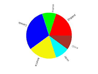
Fig.1 Pie chart created by gnuplot with assistance of python

Posts Plot a pie chart using gnuplot and Pie charting using gnuplot give new solutions of pie chart plotting and anyone interested in can take for a reference.

Saturday, October 1, 2011

Round corner rectangle in gnuplot

A simple rectangle always looks too hard while a round corner rectangle looks more comfortable. In this article I will talk about how to create an round corner rectangle in gnuplot.

There is rectangle object in gnuplot, but unfortunately there seems no option to set it a round corner one. So an absolutely new method will be used. I will use plot style "filledcurve" to create an round corner rectangle. Now come to the script.
###############################################
#Variables:
##(a,b) is the low left vertex of the rectangle
##(c,d) is the up right vertex of the rectangle
##rx is the radius along x-axis
##ry is the radius along y-axis
##x is the independent variable of the curve
f_low(a,b,c,d,rx,ry,x)=a<x && x<a+rx ? \
     -ry*sqrt(1-((x-a-rx)/rx)**2)+b+ry : \
     a+rx<x && x<c-rx ? b :c-rx<x && x<c ?\
     -ry*sqrt(1-((x-c+rx)/rx)**2)+b+ry : 1/0
#The low curve of a round corner rectangle
f_up(a,b,c,d,rx,ry,x)=a<x && x<a+rx ?\
     ry*sqrt(1-((x-a-rx)/rx)**2)+d-ry : \
     a+rx<x && x<c-rx ? d :c-rx<x && x<c ?\
     ry*sqrt(1-((x-c+rx)/rx)**2)+d-ry : 1/0
#The up curve of a round corner rectangle
###############################################
unset border    #no border
unset tics    #no tics
set sample 1000
set xrange [-10:10]
set yrange [-10:10]
set term png
set output "round_corner_rectangle.png"
plot '+' u 1:(f_low(-10,-10,10,10,1,2,$1)):\
     (f_up(-10,-10,10,10,1,2,$1)) w filledcurve\
     lc rgb"pink" notitle
#plot a round corner rectangle 
Load the plotting script, and we get picture file found_corner_rectangle.png like this.
Round corner rectangle created using filledcurve plot style in gunplot
Creative Commons License
Except as otherwise noted, the content of this page is licensed under a Creative Commons Attribution-NonCommercial-NoDerivs 3.0 Unported License.